Sampling frequency can be a confusing component of building a time waveform. What makes it confusing for many analysts who are learning Level III concepts is that it is always described in conjunction with a number of samples, resolution, and bandwidth. For this article, we will only focus on breaking out this one simple concept.
Time Waveform Basics
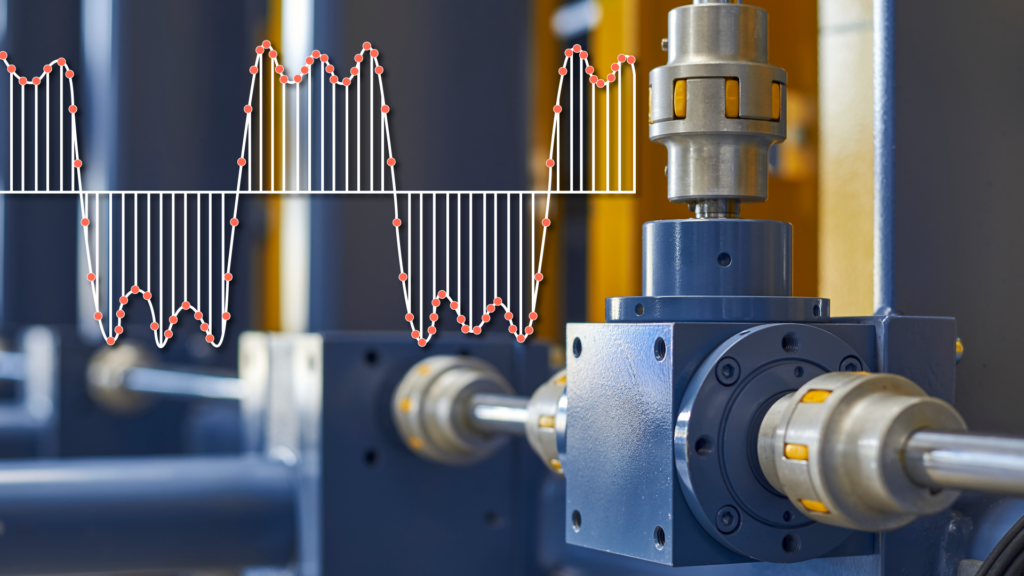
When viewing the time waveform, it appears as a single squiggly line; however, it is a number of values drawn together (dot-to-dot). The values are gathered with the data collector at a specific frequency that is built through the analysis software. The data collector acts like a voltmeter, registering these values at a set frequency. Using 256hz, for example, means that the data collector looks for a value 256 times per second and plots the value on the time waveform.
Optimal Sampling Frequency
Where this really matters is in looking at what we want to be able to view in the data. It is common to do math to calculate how many samples will be taken per tooth mesh on a gearbox, which allows us to see a cracked or broken tooth. For example, if we want a set number of samples per vane pass or another fault frequency. Without the proper sampling frequency, we cannot see some of the information necessary to make a confident call while performing our analysis.
This is an oversimplified explanation of the concept of sampling frequency, as you will not be able to calculate data points per tooth without also including the number of samples in the formula. Sampling time is simply the amount of time you want to spread out the set sampling frequency data across. For example, if I have a reading set to collect at 256hz sampling frequency and the number of samples set at 256, I will collect one second of time waveform data. If I set the sampling frequency at 256hz and the number of samples at 512, I will get a ½ second of data.
This knowledge can give you the math required to capture a specific number of samples per event in the system, allowing you to collect valuable data.


4 Comments
“For example, if I have a reading set to collect at 256hz sampling frequency and the number of samples set at 256, I will collect one second of time waveform data. If I set the sampling frequency at 256hz and the number of samples at 512, I will get a ½ second of data.”
At 256Hz we collect 256 samples/ second so if you collect 512 samples you would get 2 seconds of data would you not?
This article is misleading at best. First of all, most data collectors use a sampling frequency at least 2.5 times higher than the desired bandwidth (Nyquist theorem), so if you set a sampling frequency of 256 Hz, you are actually getting a usable bandwidth of around 100 Hz. This would mean the data you’re trying to sample, if indeed is at 256 Hz, would not even show up as it is completely undersampled. Second, you need to oversample at least ten times any expected frequency component. Thus if you have a suspected 256 Hz frequency component, the sampling rate should be at least 2,560 Hz. Higher is better, 10X is the minimum recommended.
Yes, that’s correct.
This would be true if the focus of the article was to create an fft spectrum from the time waveform. I really like your comment, but the intention is focused on ONLY creating your setup for the time waveform – which involves different criteria.
Of course you want to oversample, and if you ignore nyquist you will get aliasing in the FFT – there are data collection and analysis softwares in which you create the time waveform setup and fft’s independently.
The article is not misleading, I apologize for any confusion this may have caused.